Graphs
Terminology
Nodes
Also known as Vertices
Nodes are the points in a network graph that edges connect to. They can display or represent people, places or any object
- We denote the vertex set of a graph $G$ by $V(G)$
- A pair of vertices $V_i$ and $V_j$ in $V$ are adjacent if they are connected by an edge .
- Adjacency requires a edge between two nodes
- The number of adjacent nodes [of a vertex] is called the degree
Isolated node
A node with no edges
- Has a Degree of 0
Root node
The starting node. Semantically ambiguous, as the root node can imply the starting node of a decision tree, (or any graph) which is correct. But it can also be associated or interchanged with source nodes, which is not preferred.
Source node
- No incoming edges
- Only outgoing edge(s)
Sink node
- No outgoing edges
- Only incoming edge(s)
Leaf node
A node of degree 1. Only used when referring to trees.
Neighbourhood
The neighbourhood of a vertex $v$ is the set of vertices adjacent to $v$.
Order
The number of vertices in a graph.
Edges
Edges are the lines in-between nodes that display a connection between nodes. Edges represent connections, relations or any logical path.
- We denote the edge set of a graph $G$ by $E(G)$
Incidence
An incidence is a pair $(u,e)$ where $u$ is a vertex, and $e$ is an edge incident to $u$
If the vertex $u$ is connected to $e$; $e$ is an edge incident to $u$
Wikipedia definition
In graph theory, a vertex is incident to an edge if the vertex is one of the two vertices the edge connects.
An incidence is a pair $(u,e)$ where $u$ is a vertex and $e$ is an edge incident to $u$.
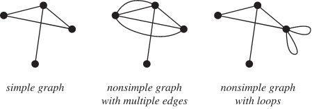
Loops
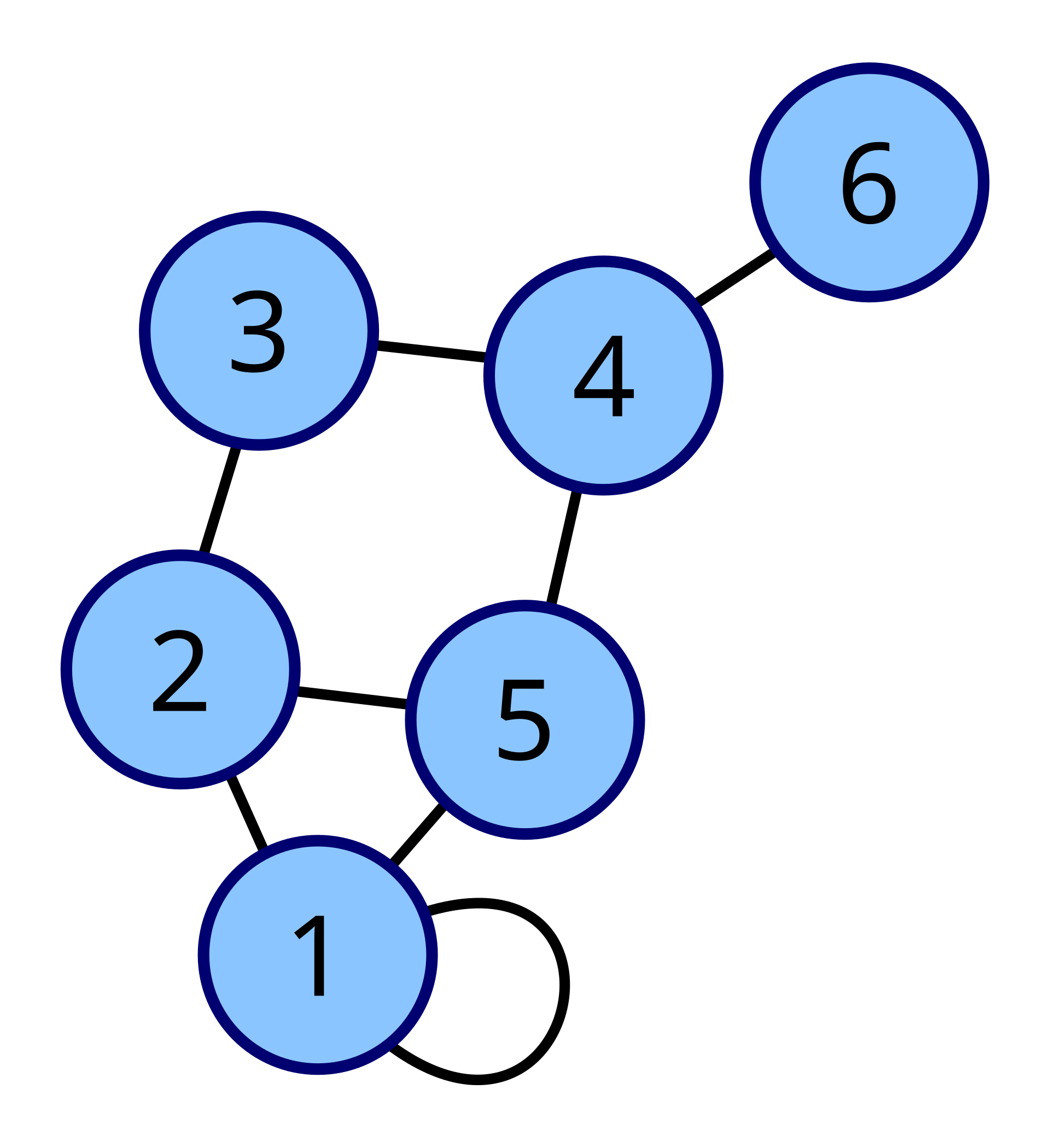
A loop is an edge that has the same starting and ending node. See node 1 below:

Paths
A path is the route from one vertex to another. A path can contain many edges, or a single. it depends on what nodes are being selected.
- Vertices cannot repeat
- Edges cannot repeat
Note
- Check out Euler paths and Euler circuits:
- Check out Hamiltonian Paths
Euler Path
A path that uses each edge once only without returning to starting vertex is an Euler path.
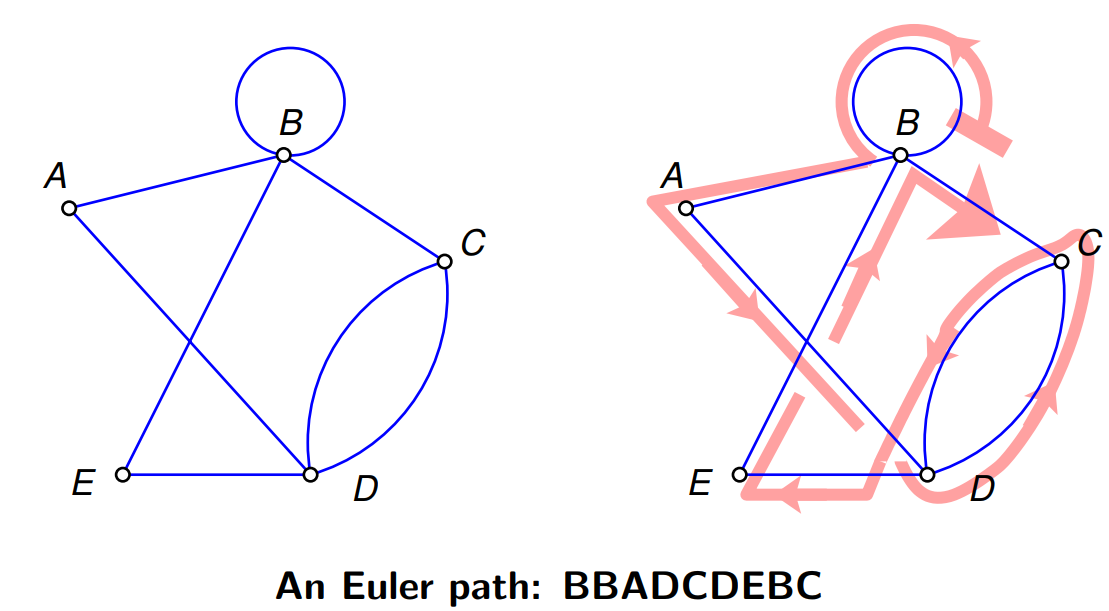
- Doesn't return to starting vertex
- Can pass through nodes more than once.
- Don't exist if a graph has more than two vertices of odd degree.
- Exists if all vertices of a graph have even degree.
- Exists if a connected graph has exactly two odd vertices. The starting point must be one of the odd vertices and the ending point will be the other of the odd vertices.
Euler circuit
A path that uses each edge once only and returns to starting vertex is an Euler circuit.
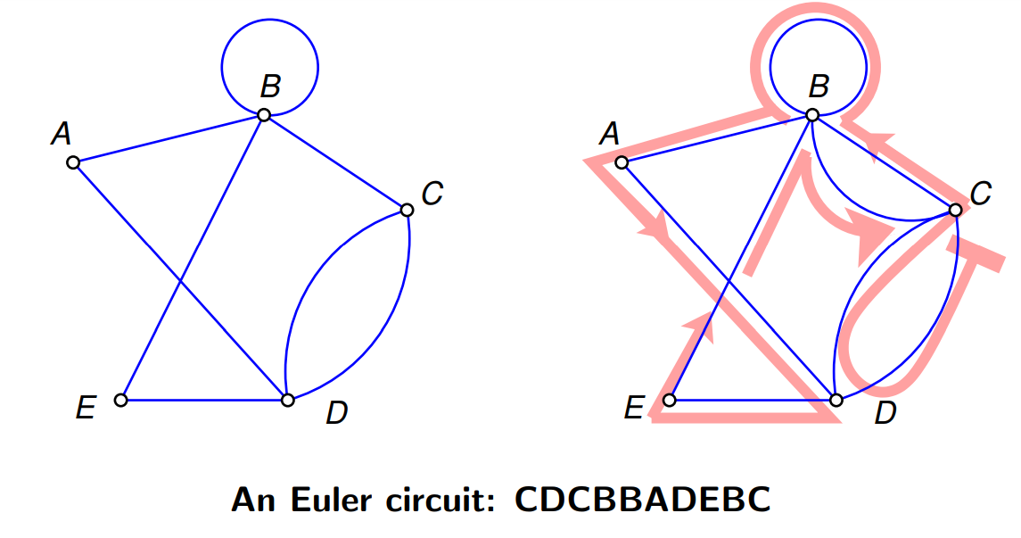
If an undirected graph $G$ is connected and every vertex (not isolated) in $G$ has an even degree, then $G$ has an Euler circuit.
- Uses each edge once
- Does return to starting vertex
Hamiltonian Path
A path that passes every vertex exactly once without returning to starting vertex is an Hamiltonian path.
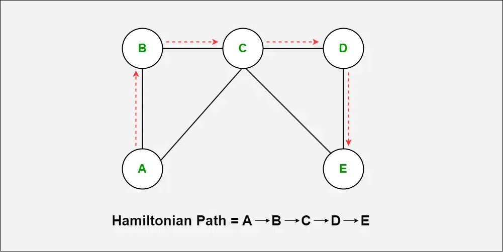
- Uses every node once
- Doesn't return to starting node
- Don't have to traverse every edge
Hamiltonian Circuit
Note
This is used very often in this course. See Travelling salesmen problem
Important
A cycle and a circuit are different. But the properties of both Hamiltonian cycles and Hamiltonian circuits are the same. Hence they reffer to the same thing.
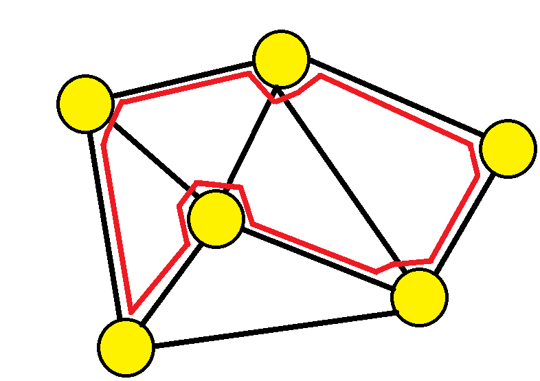
A path that passes every vertex exactly once and returns to the starting vertex is an Hamiltonian path.
- Uses every node once
- Does return to starting node
Path graph
A graph that is a path across the diameter

Transitive closure
Is there a path from $A$ to $B$ ?
The transitive closure of a graph is a graph which contains an edge between $A$ and $B$ whenever there is a directed path from $A$ to $B$. In other words, to generate the transitive closure every path in the graph is directly added as an additional edge.
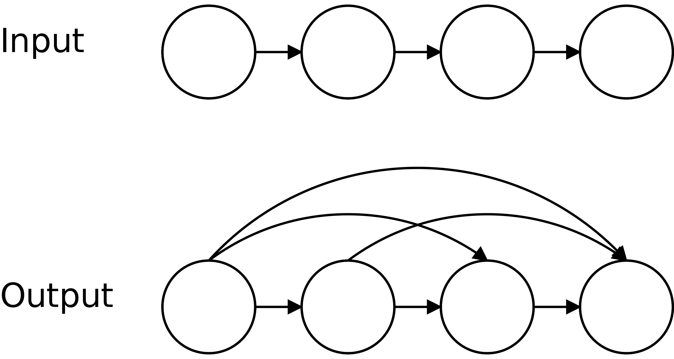
A graph $G^*$ which is the transitive closure of $G$ will have a directed edge to every node it can traverse to.
Undirected Graphs
Undirected graphs have edges that can be travelled along in any direction.
Directed Graph
Also known as a digraph.
Bassically just the same as a regular undirected graph, but the edges have arrows (direction). Formally, a digraph is an ordered pair G = (V, E) of edges $(x,y)$ of arrows "from $x$ to $y$".
Where:
- $x$:
- Is the tail
- Is the direct predecessor of $y$
- $y$:
- Is the head
- Is the direct successor of $x$
If a path leads from $x$ to $y$, then $y$ is said to be a successor of $x$ and reachable from $x$, and $x$ is said to be a predecessor of $y$.
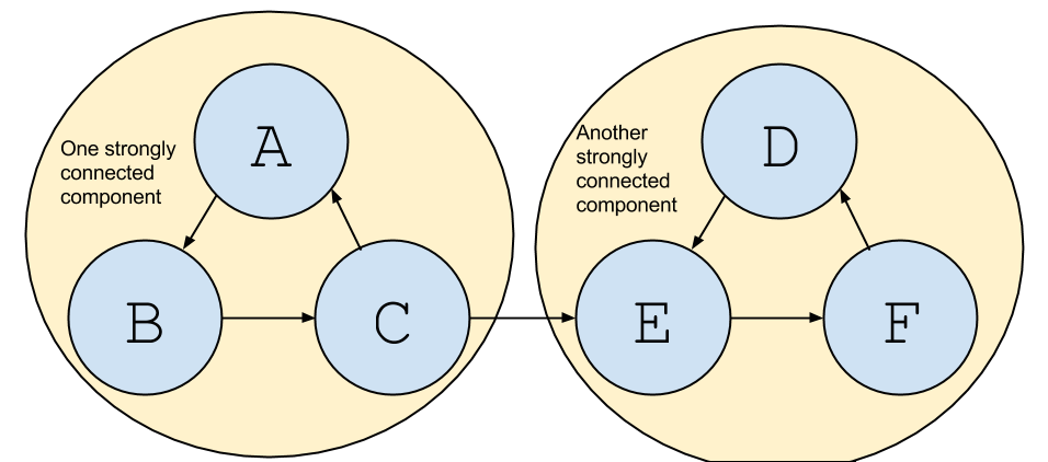
Strongly Connected Digraph
A directed graph $G$ is strongly connected if there is a directed path from every vertex to every other vertex in $G$.
Dag / DAGS
A Directed Graph with no directed cycles
- I.e. An Acyclic Directed Graph
Degree
The degree of a node is the number of edges that come off it.
- Note that a node of degree zero is called an Isolated node
Cycle
A cycle in a graph is a path that returns to the starting node.
- Vertices cannot repeat
- Edges cannot repeat
- Loops back to original vertex (repeats on one node)
Acyclic
Does not contain any cycles.
Circuit
A circuit in a graph is a path that returns to the starting node.
- Vertices may repeat
- Edges cannot repeat
- Loops back to original vertex (repeats on one node)
Walk
- Vertices may repeat
- Edges cannot repeat
- Loops back to original vertex If it wants to (repeats on one node)
Trail
- Vertices may repeat
- Edges cannot repeat
Graph definition
A graph $G$ is a finite non-empty set of objects called vertices or nodes which are connected by edges.
Measures of Similarity
The similarity measure is the measure of how much alike two data objects are. Similarity measure in a is a distance with dimensions representing features of the objects. If this distance is small, it will be the high degree of similarity where large distance will be the low degree of similarity.
Two main consideration about similarity:
Similarity = 1 if $X = Y$ (Where $X$, $Y$ are two objects) Similarity = 0 if $X \neq Y$
Warning
I have never seen cosine simularity anywhere. Don't worry too much about it
Best example in the world:
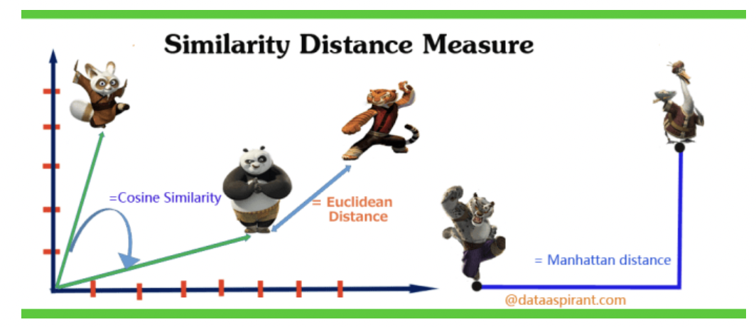
Distances
Topological distance
The number of edges in the shortest path connecting 2 nodes. For unweighted graphs, each edge has a nominal distance of 1.
Euclidian distance
The most commonly understood distance metric
Euclidean Distance is the straight line distance between two entities. Which is worked out using Pythagoras Theorem
When data is dense or continuous, this is the best proximity measure.
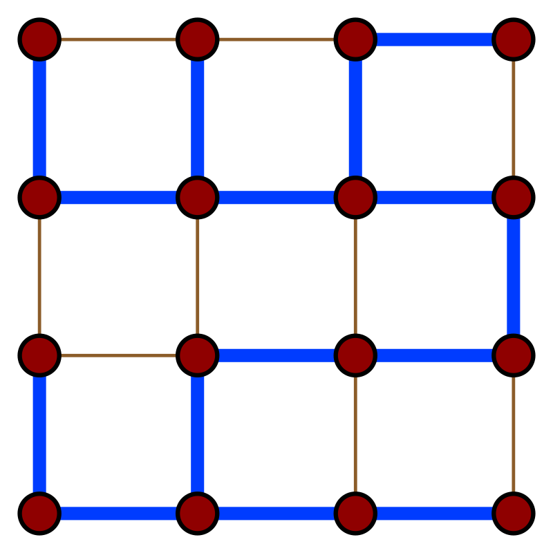
Manhattan distance
Manhattan Distance is the distance restricted to traversal via a street grid between two entities. Which is worked out by adding the vertical and horizontal cells traversed.
In a simple way of saying it is the total sum of the difference between the x-coordinates and y-coordinates.
The heuristic function for distance calculation

Which is the absolute cell distance in the $x$ direction plus the absolute cell distance in the $y$ direction. The absolute value is always positive.
Cosine similarity metric
Finds the normalised dot product of the two attributes. By determining the cosine similarity, we would effectively try to find the cosine of the angle between the two objects. The cosine of 0° is 1, and it is less than 1 for any other angle. It is thus a judgement of orientation and not magnitude: two vectors with the same orientation have a cosine similarity of 1, two vectors at 90° have a similarity of 0, and two vectors diametrically opposed have a similarity of -1, independent of their magnitude.
Topological sort
- Directed graphs
- Chop the source nodes of each iteration
Also known as a topological ordering
In computer science a topological sort or topological ordering of a Directed Graph is a linear ordering of its vertices such that for every directed edge uv from vertex u to vertex v, u comes before v in the ordering.
A topological ordering is possible iff the graph has no directed cycles, that is, if it is a directed acyclic graph (Dag - DAGS).
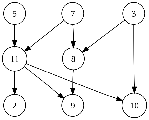
The graph shown above has many valid topological sorts, including:
- 5, 7, 3, 11, 8, 2, 9, 10 (visual top-to-bottom, left-to-right)
- 3, 5, 7, 8, 11, 2, 9, 10 (smallest-numbered available vertex first)
- 5, 7, 3, 8, 11, 10, 9, 2 (fewest edges first)
- 7, 5, 11, 3, 10, 8, 9, 2 (largest-numbered available vertex first)
- 5, 7, 11, 2, 3, 8, 9, 10 (attempting top-to-bottom, left-to-right)
- 3, 7, 8, 5, 11, 10, 2, 9 (arbitrary)
This can be calculated through Kahn's Algorithm
Kahn's Algorithm
A Topological sort algorithm, first described by Kahn (1962), works by choosing vertices in the same order as the eventual topological sort. First, find a list of "start nodes" which have no incoming edges and insert them into a set $S$; at least one such node must exist in a non-empty acyclic graph. Then:
L ← Empty list that will contain the sorted elements
S ← Set of all nodes with no incoming edges

while S is non-empty do
    remove a node n from S
    add n to tail of L
    for each node m with an edge e from n to m do
        remove edge e from the graph
        if m has no other incoming edges then
            insert m into S
if graph has edges then
    return error (graph has at least one cycle)
else
    return L (a topologically sorted order)
Graph Diameter and radius
Note
Note that the diameter is the max graph ecentricity. The radius of the graph requires a center point to be defined
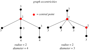
The longest shortest path between any two nodes counted by edge and weights.
Also defined as the largest distance between any pair of vertices.
- A disconnected graph has a diameter of $\infty$
The examples below have a diameter of 2 (2 edges to traverse to get from a to b):
- A graph of one vertex has diameter 0
Example:
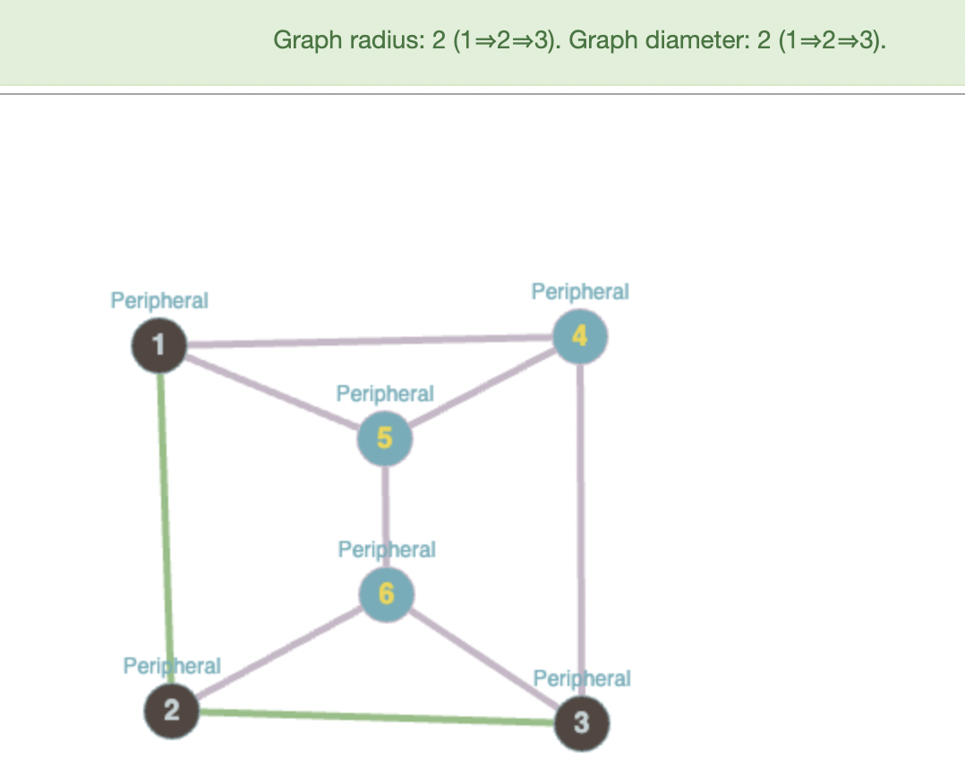
*Note that the radius and diameter is counted by the number of edges
Network graphs
Graph
A graph $G=(V,E)$ is made up of a set of vertices/nodes ($V$) and a set of lines called edges ($E$) that connect the vertices or nodes.
- $|V|$ is the number of vertices in the graph
- $|E|$ is the number of edges in the graph.
Example
Example: Using Graph Notation to define a Graph: - $V={A,B,C,D,E}$ - $E={A-B,A-C,A-D,A-E,B-C,B-D,B-E,C-D,C-E,D-E}$ - $G=(V,E)$ - $|V|$ returns 5 - There are 5 nodes or vertices - $|E|$ returns 10 - there are 10 edges in this graph
Sub graph
A graph $H$ is a subgraph of $G$ if $V(H) \subset V(G)$ and $E(H) \subset E(G)$.
We can then obtain $H$ from $G$ by deleting edges and or vertices from $G$.
Simple graph
A simple graph, also called a strict graph is an unweighted, undirected graph containing no graph loops or multiple edges.
A simple graph may be either connected or disconnected. Unless stated otherwise, the unqualified term "graph" usually refers to a simple graph.
For simple connected graphs the amount of edges you can have are striclty bounded. The number of edges will always be between the arrangement of a tree or a complete graph:
$$ \overset{\text{(trees)}}{(|V|-1)} \le |E| \le \overset{\text{(complete graphs)}}{\left(\frac{|V|(|V|-1)}{2}\right)} $$
Multigraph
A graph that can have multiple edges between the same pair of nodes. In a road network this could, for example, be used to represent different routes with the same start and end point.
Connected Graph
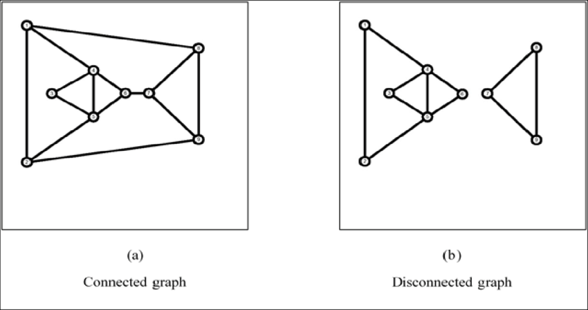
A graph where all nodes are connected
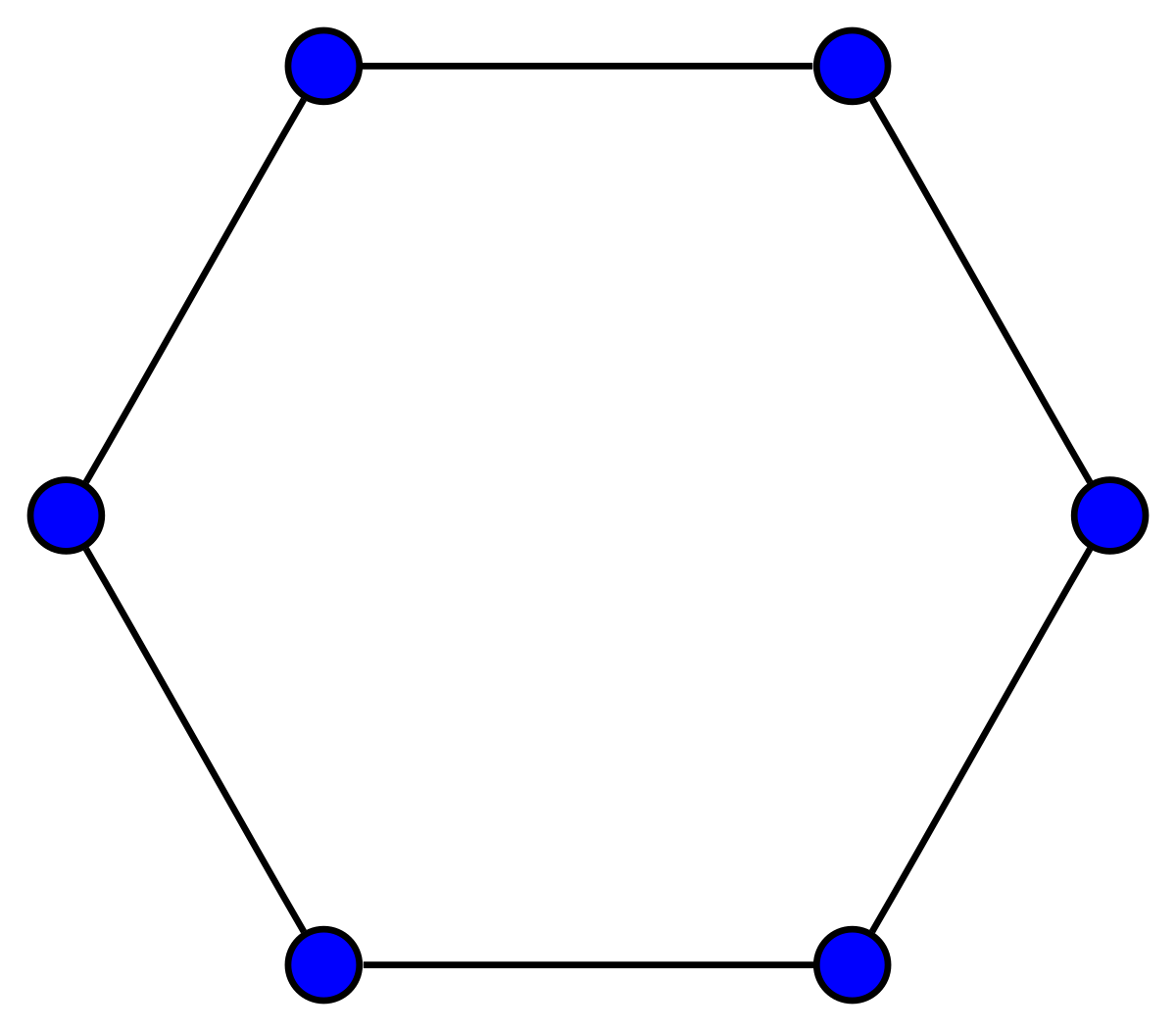
Ring Graph
Also known as a Cycle Graph A graph that forms a ring
- All nodes have a degree of 2
Disconnected Graph
A graph where not all nodes are connected.
Bridge
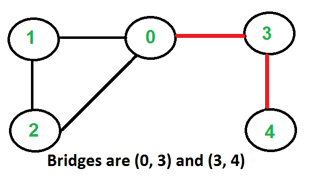
A bridge is an edge that if deleted would cause the graph to become disconnected.
Cut Node
A Cut Node is an node that if deleted would cause the graph to become disconnected.
Cyclic Graph
A graph where a cycle can be formed.
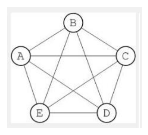
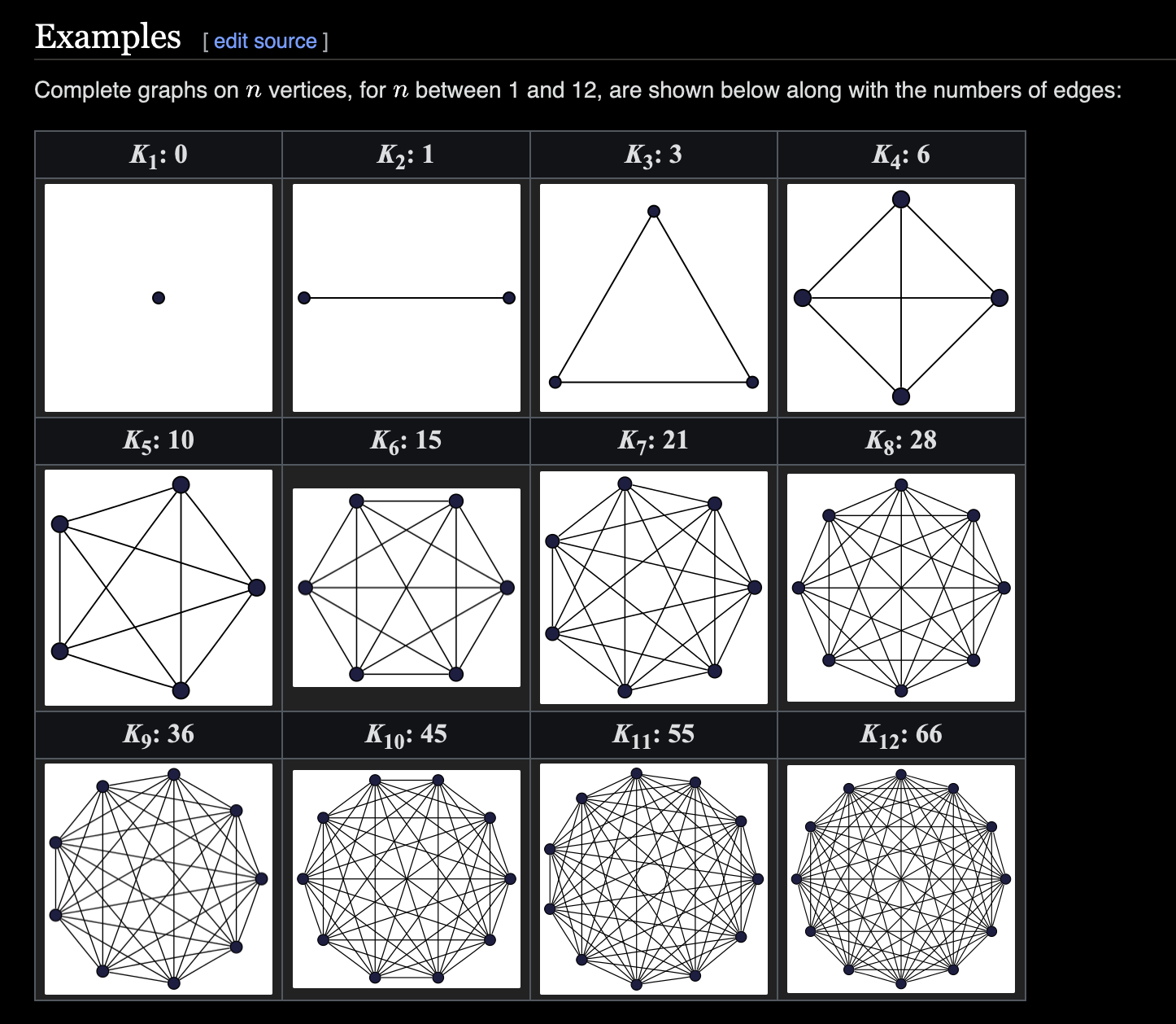
Complete Graphs
- A complete graph has every pair of vertices joined by one edge.
- i.e. Every node is connected together by an edge
A complete graph with $n$ vertices will have a degree of $(n-1)$ for all nodes, and a total of $\frac{n(n-1)}{2}$ edges
For $n$ nodes we usually abbreviate it as $Kn$. For example, $K4$ is the complete graph with four nodes:
The diameter of a complete graph is 1
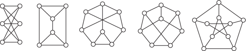
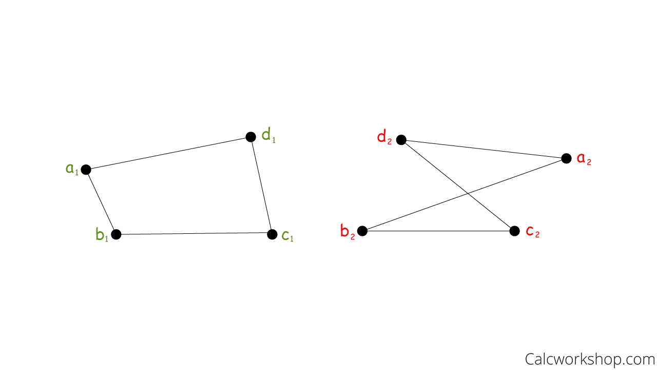
Isomorphic Graphs
Also known as topologically equivalent graphs.
Graphs or networks that look different but represent the same information are said to be topologically equivalent or isomorphic.
Isomorphic Graphs have the same number of vertices, edges and connections between vertices, but may look completely different.
Bipartite Graphs
A graph $G$ is bipartite if its vertices can be partitioned into two sets $X$ and $Y$ , called partite sets, such that every edge in $E(G)$ is between a vertex in $X$ and a vertex in $Y$ .
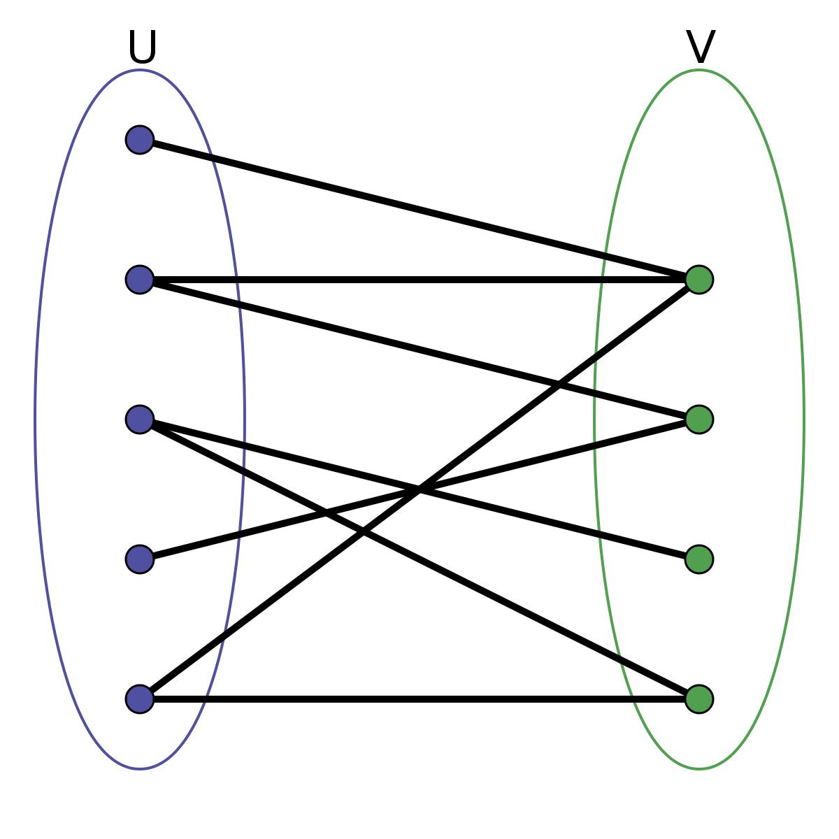
As shown above, bipartite graphs have a chromatic number of 2
Trees
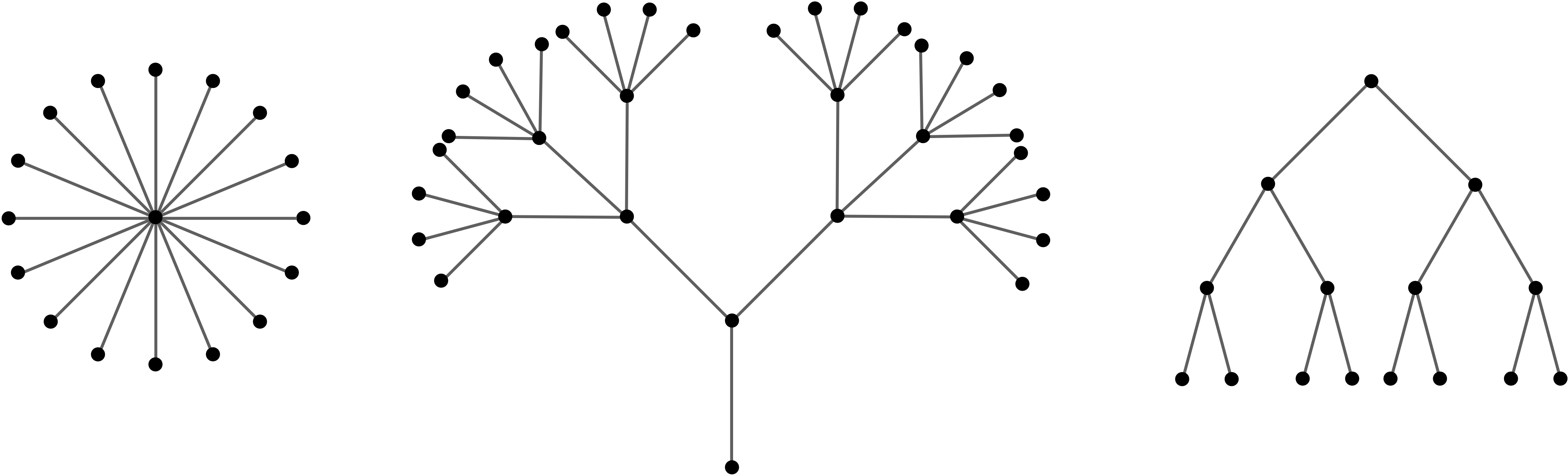
For any tree $T = (V, E)$ with $|V|$ = $n$, $|E| = n − 1$. As an extension, can you figure out how many edges there are in a forest?
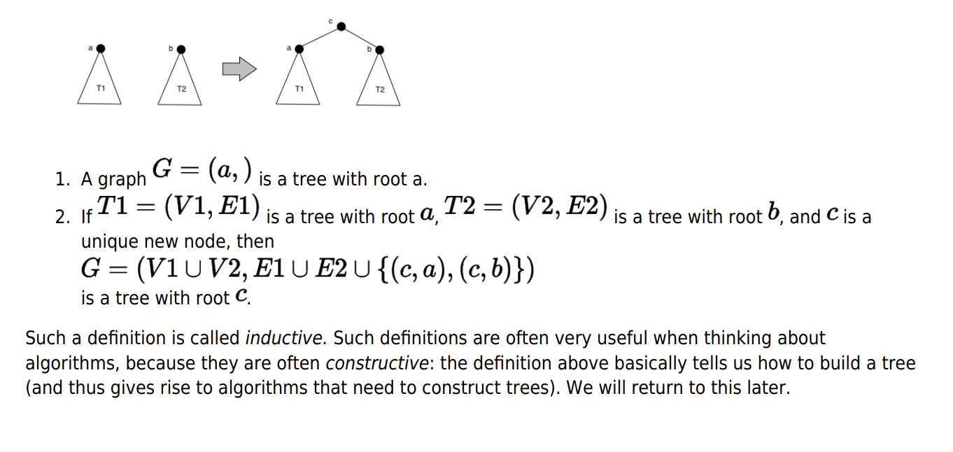
Formal definition of a tree
Or the "Inductive"
Spanning Tree
A spanning tree is a connected graph that has no circuits or cycles (Acyclic).
If a graph has $n$ vertices its spanning tree it will have $(n-1)$ edges.
Minimum amount of edges to connect all nodes
Minimum Spanning Tree
A minimum spanning tree is a spanning tree for a weighted graph whose edges add up to the smallest possible value.
- Found via Prim's algorithm
A graph can have several minimum spanning trees. For example if we replace all the weights with $1$ in a graph with $n$ vertices. The resulting graph will have $n$ minimum spanning trees.
If all the edge weights of a given graph are the same, then every spanning tree of that graph is minimum.
Spanning Subgraph
A Spanning Sub graph $H$ of a graph $G$ is a sub graph of $G$ such that $V (H) = V (G)$.
Decision tree
A tree where each non-leaf node splits off to two other child nodes. If there is one source node, the tree has $n$ vertices and $n - 1$ edges.
Random decision forests
Or decision forests, have $n - s$ edges. For $n$ vertices and $s$ source nodes. See my discussion. Also the same amount of edges in a regular forest.
Binary tree
A type of Decision tree, but with the absence of the decision abstraction, and it's literally just 0,1 or 2 children per parent for the entire graph

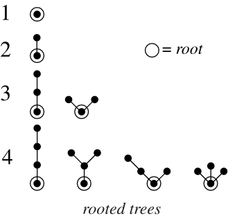
Rooted tree
A rooted tree is a tree in which a special ("labeled") node is singled out. This node is called the "root" or (less commonly) "eve" of the tree. Rooted trees are equivalent to oriented trees
Forest
A graph with no cycles. More specifically, a disconnected graph, where each connected component is a tree.
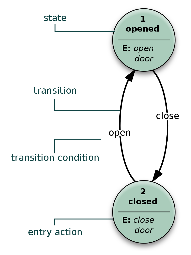
State Diagrams
A Directed Graph showing connections between states of objects or abstract instances
Colouring
Vertex Colouring
Also known as Chromatic Colouring
- Adjacent nodes cannot be the same colour
- Usually used to represent nodes of conflict
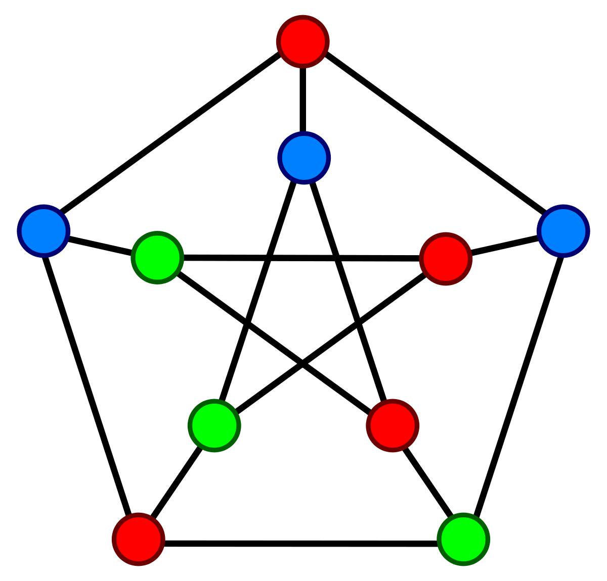
The chromatic number of this graph is 3. As there are 3 unique colours.
Chromatic Number
The chromatic number of a graph $G$ is the minimum value $k$ for which a $k$-colouring of $G$ exists.
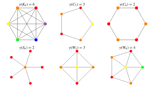
See example Vertex Colouring
Math
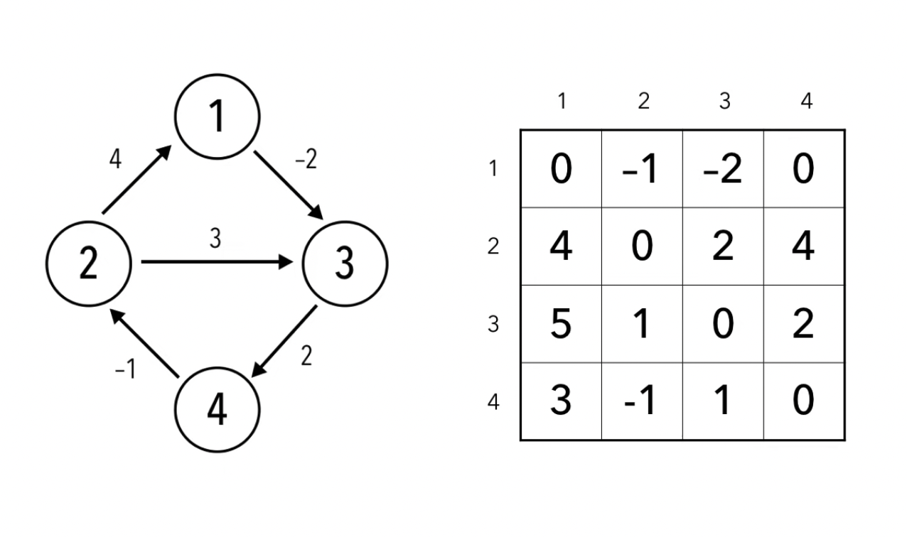
Adjacency Matrix
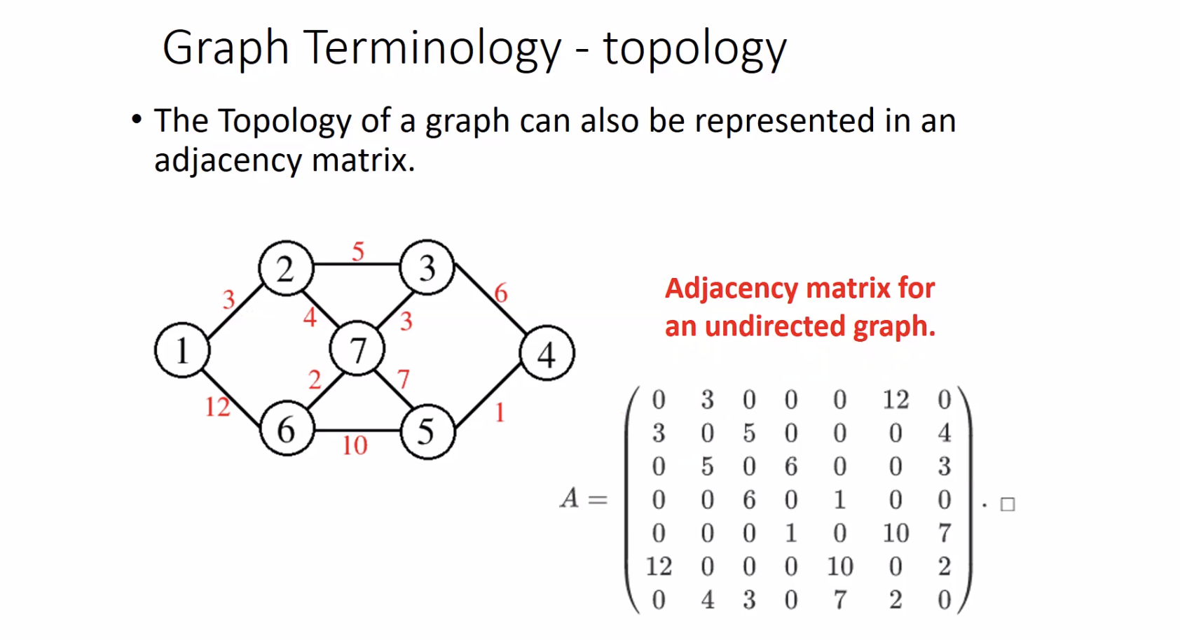
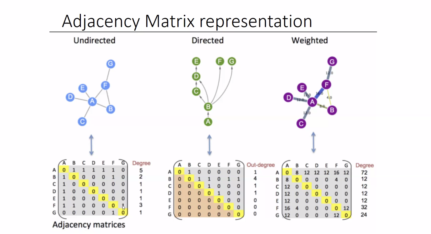
An adjacency matrix shows weightings of edges on an undirected graph. Where an adjacency matrix of $1$s and $0$s is not weighted, and identifies an edge.
An example of an undirected connected graph with nodes $A$,$B$, and an edge between them
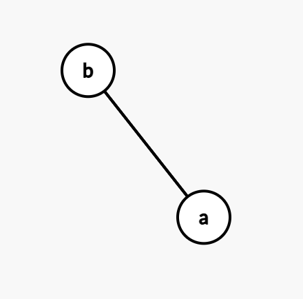
$$ \begin{array}{c|cc} & A & B \newline \hline A & 0 & 1 \newline B & 1 & 0 \end{array} \hspace{0.6cm} \text{or equivalently} \hspace{0.6cm} \begin{bmatrix} 0 & 1 \newline 1 & 0 \end{bmatrix} $$
A directed graph where $A \to B$:
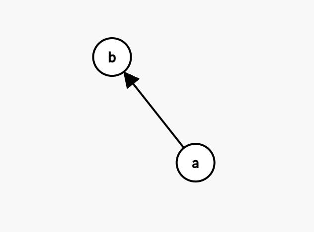
$$ \begin{array}{c|cc} & A & B \newline \hline A & 0 & 1 \newline B & 0 & 0 \end{array} $$ The direction can be read from the left of the matrix (left side of rows) to the right of the row to find the head.
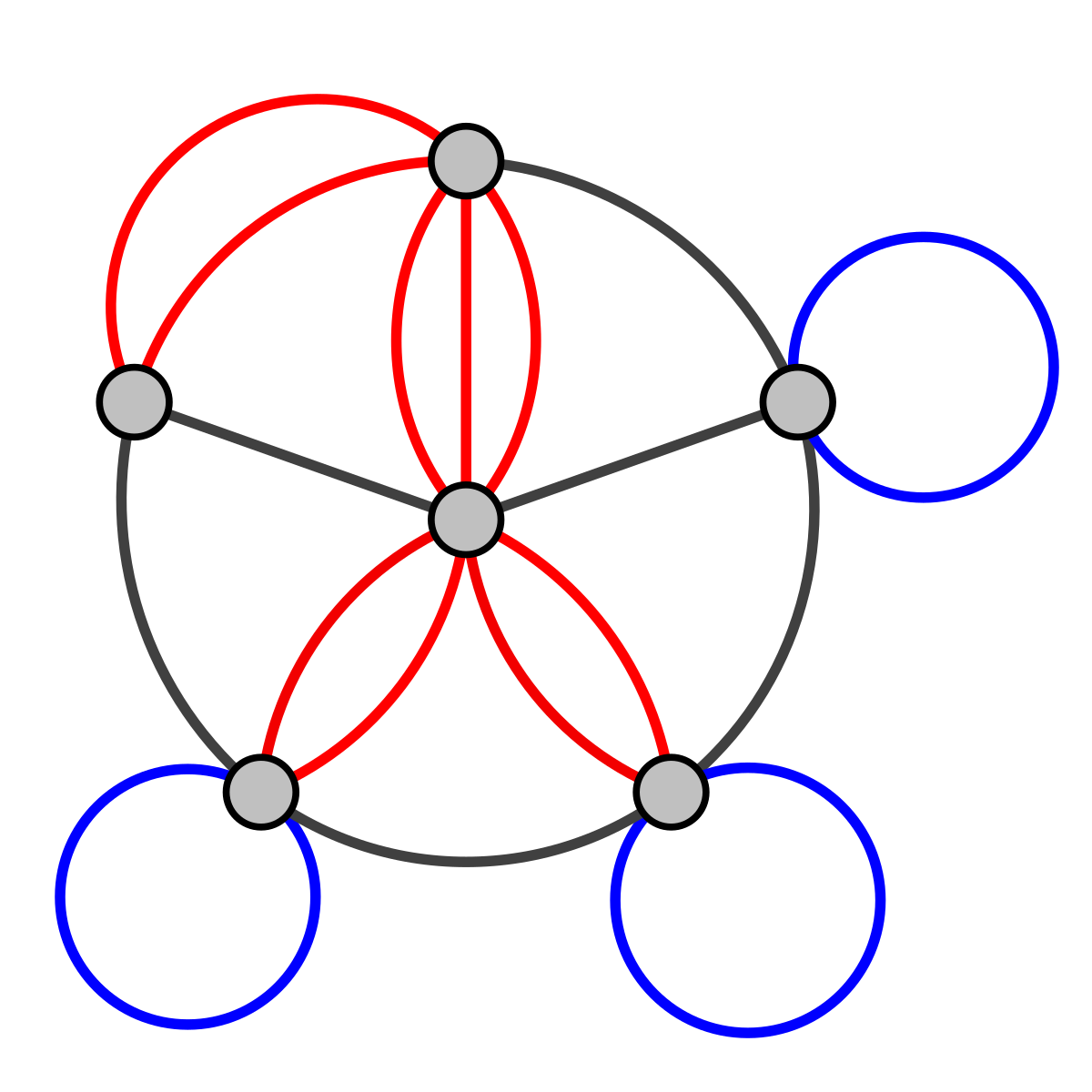
Note
- Undirected graphs are diagonaly symetrical with respect to the rows and collums of an adjacency matrix. Directed graphs are not
- For graphs with no loops (e.g. simple graphs) All adjacency matricies are empty on the diagonal. An example of a graph with loops:
$
\displaystyle {\begin{pmatrix}2&1&0&0&1&0\newline1&0&1&0&1&0\newline0&1&0&1&0&0\newline0&0&1&0&1&1\newline1&1&0&1&0&0\newline0&0&0&1&0&0\end{pmatrix}}
$. 
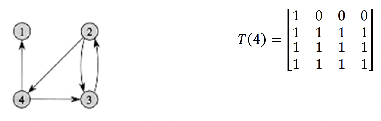
Transitive closure matrix
A matrix $(i,j)$ where $1$ represents a valid path from $i$ to $j$, and $0$ otherwise. Where $i$ to $i$ is considered connected $1$.
Incidence Matrix
For its simplest form we identify the nodes of a directed graph with numbers $1…n$ and give a matrix $M$ of zeros and ones such that:
$$M_{ij} = \begin{cases} 1 \text{ if } i \text{ and } j \text{ are connected} \ 0 \text{ otherwise} \end{cases} $$
Distance Matrix
The shortest distances from $A$ to $B$ for each pair of nodes in a graph. Used in the Floyd-Warshall algorithm
Adjacency List
A list of adjacent nodes:
$$ \begin{align} A &= {B,C} \newline B &= {A} \newline C &= {A} \end{align} $$
Searching graphs
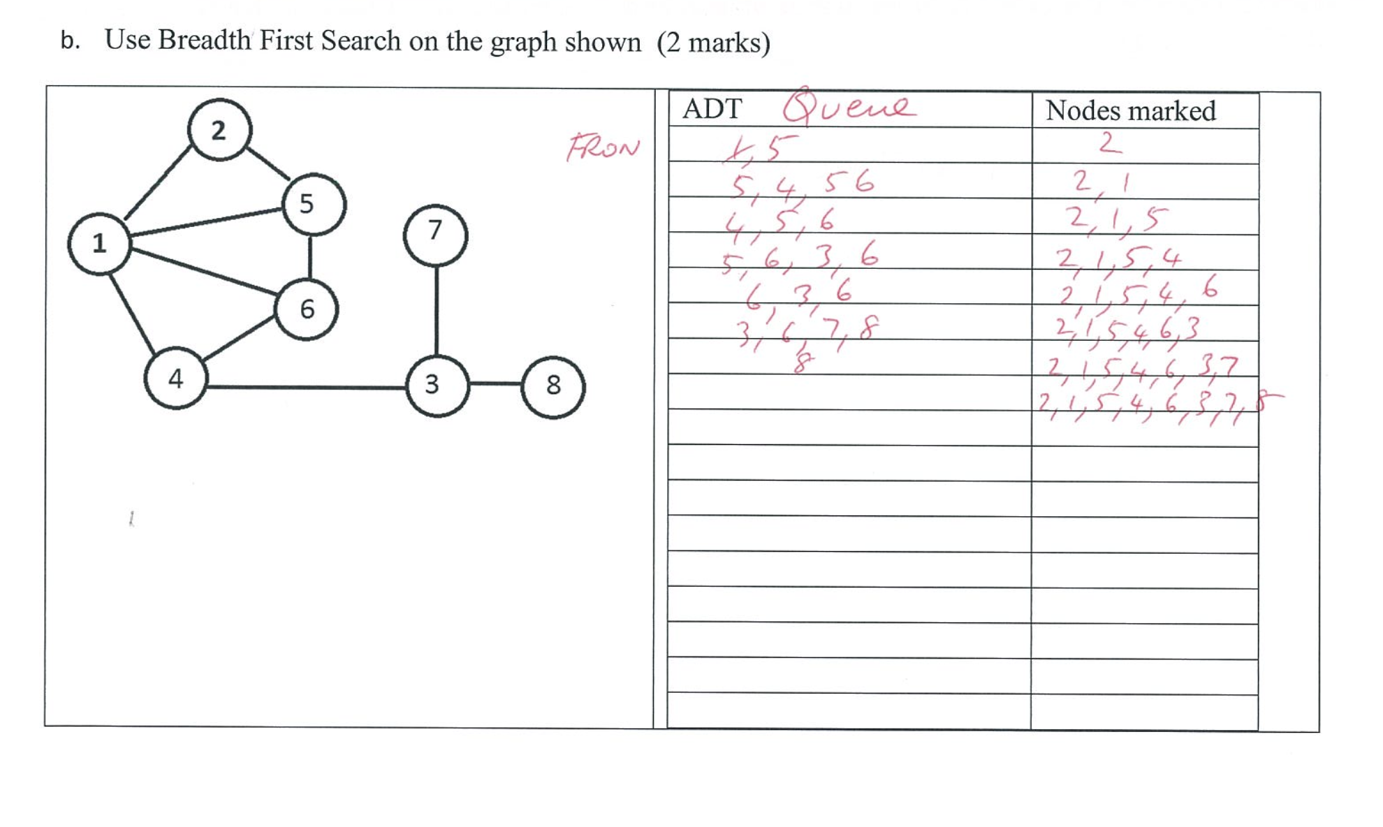
BFS Breadth First Search
Quote
"The basic idea of breadth-first search is to fan out to as many vertices as possible before penetrating deep into a graph. "A more cautious and balanced approach."
Main points:
- To see if a node is connected to another
- Uses a queue to keep track of nodes to visit soon
- Uses an array/set called
seento mark visited vertices - If the graph is connected, BFS will will visit all the nodes
- A BFS tree will show the shortest path from
AtoBfor any unweighted graph
Algorithm:
- Add initial node to
queueand mark inseen- Then add it's neighbours to the queue
- Remove the next element from the
queueand call itcurrent. - Get all neighbours of the current node which are not yet marked in
seen.- Store all these neighbours into the
queueand mark them all inseen.
- Store all these neighbours into the
- Repeat from the step 2 until the
queuebecomes empty.
Gif example of BFS:
SAC example:
Uses of BFS
- Check connectivity
- Bucket-fill tool from Microsoft paint
- Finding shortest path (when modified. pure BFS will not do this)
- Diameter of a graph
- The diameter of a graph is the longest shortest path between any two nodes in a graph. Using BFS in a loop and finding the shortest path starting from every node in the graph, keep record of the longest shortest path found so far.
- Cycle detection
- Bipartite graph detection using BFS
BFS Breadth First Search can also be considered a waveform due to its nature
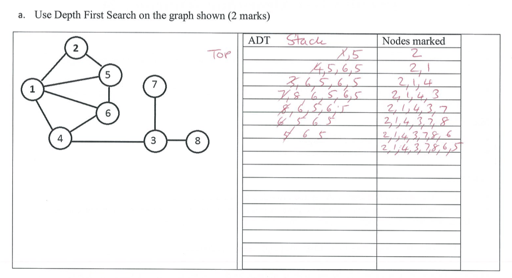
DFS Depth First Search
Quote
"The basic idea of depth-first search is to penetrate as deeply as possible into a graph before fanning out to other vertices. "You must be brave and go forward quickly."
Main points:
- To see if a node is connected to another
- Uses a
stackfor storing vertices - We do not check whether node was seen when storing neighbours in the
stack- instead we perform this checking when retrieving the node from it. - Builds a spanning tree if the graph is connected
- Creates longer branches than BFS
Algorithm:
- We add the initial node to
stack.- And then push it's neighbours onto the stack
- Pop an element from the
stackand call itcurrent. - If the
currentnode isseenthen skip it (going to step 6). - Otherwise mark the current node as
seen - Get all neighbours of the
currentnode and push them onto thestack. - Repeat from the step 2 until the
stackbecomes empty.
Gif example of DFS:

Practice example:
Uses for DFS
- Detecting cycles in a graph
- Topological sorting
- Path Finding between initial state and target state in a graph
- Finding strongly connected components
- Checking if a graph is bipartite
Tree traversal
How to search trees:
- Any tree, but normally a Binary tree
- You can use
- DFS Depth First Search
- Pre-order
- Hug the left most nodes (recursively the first (left) child in each node)
- Post-order
- Same as pre-order, but it goes depth first (prints the deepest left node), and then recursively scales back up
- In-order
- Youtube
- Go left until you cant, then print - and scale upwards
- Recursively traverse the current node's left subtree. Visit the current node (in the figure: position green). Recursively traverse the current node's right subtree.
Definition:
In computer science, tree traversal (also known as tree search and walking the tree) is a form of graph traversal and refers to the process of visiting (e.g. retrieving, updating, or deleting) each node in a tree data structure, exactly once.
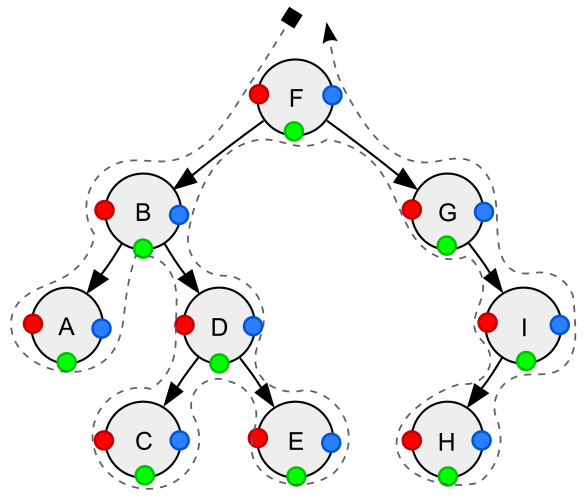
For each of these, consider how you would recursively visit each node, and that 'visiting' a node is a discrete operation and does not happen automatically when you traverse to a node.
Depth-first traversal (dotted path) of a binary tree: Pre-order (preorder) (node visited at position red 🔴): F, B, A, D, C, E, G, I, H;
preorder(node):
    if node is None:
        return
    visit(node)
    preorder(node.left)
    preorder(node.right)
In-order (node visited at position green 🟢): A, B, C, D, E, F, G, H, I;
norder(node):
    if node is None:
        return
    inorder(node.left)
    visit(node)
    inorder(node.right)
Post-order (node visited at position blue 🔵): A, C, E, D, B, H, I, G, F.
postorder(node):
    if node is None:
        return
    postorder(node.left)
    postorder(node.right)
    visit(node)
Spanning trees / forests
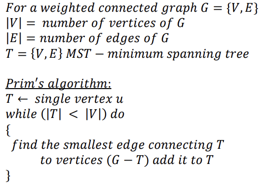
Prim's Algorithm
A greedy algorithm used to find the minimum spanning tree
Online tool
Algorithm
- Begin at any vertex
- Select the cheapest edge emanating from any vertex you've visited so far. If the edge forms a cycle discard it and select the next cheapest.
- Draw an edge to that node and consider it visited
- Repeat until all vertices have been selected.
Example:
Pseudocode:
Pick any vertex and add it to "vertices" list

Loop until ("vertices" contains all the vertices in graph)
    Select shortest, unmarked edge coming from "vertices" list
    If (shortest edge does NOT create a cycle) then
        Add that edge to your "edges"
        Add the adjoining vertex to the "vertices" list
    Endif
    Mark that edge as having been considered
EndLoop
Or
Prim's algorithm for finding an MST is proved to produce a correct result
Kruskal's algorithm
Note
Just for fun. Not in the study design
Finds minimum spanning forest by connecting the shortest edges in the graph. Works like prims, but orders the list of edges from shortest to longest and builds a tree that way
Shortest Path algorithms
Quickest way to get from $A$ to $B$. Usually by shortest weight.
Dijkstra's algorithm
Pronounced Dike-stra. Finds the shortest greedy path via a priority queue.
- Although dijkstras does store information as it is building a solution, it is not Dynamic Programming because it does not explicitly or fully solve any discrete sub-problems of the original input. This is debated, but for the sake of VCE just remember it as greedy
Note
For your exam, you don't need to remember how a heap works or the intracacies of the time complexities below. Just remember that there's 2 time complexities and they differ based on implimentation. Maybe learn how to justify one of them in case you need to write a proof.
Worst case performance if using a priority queue (Fibonacci heap version): $$ \boxed{\displaystyle O(|E|+|V|\log |V|)} \newline \text{or equivalently,} \newline \displaystyle O(|V|\log(|V|+|E|)) $$
This is because you're initialising each node into unexplored. Which is both $O(|V|)$ and setting the size of unexplored to $|V|$ which means the while loop will run at most $O(|V|)$ times. And the pop operation for a vertex with with minimum distance from the priority queue (Fibonacci heap) is $O(\log |V|)$. Which means you are running $O(|V| \log |V|)$ operations there.
Then considering the inner loop of for each neighbour N of V do, you can't immediately think of it as having that automatic coeficcient of $|V|$ because it's in that while loop. Instead, think of it on a higher level and what it's doing overall. That loop is the mechanism for relaxing edges if you find a shorter path. And when you run the algorithm you will see that relaxation is done once per edge1. So that contributes the extra term of $O(|E|)$ for a final time complexity of $O(|V|\log(|V|+|E|)) \equiv O(|E|+|V|\log |V|)$
Worst case performance when using an array:
$$ \boxed{ \displaystyle O(|V|^2) } $$
When using an array, Dijkstra's algorithm must loop over all nodes to pick the next closest node. This is clearly a lot slower than using a priority queue, where that operation can be done much faster (e.g. $ O(\log |V|) $).
The initial naive time complexity is:
$$ O(|V|^2 + |E|) $$
- The $ O(|V|^2) $ comes from scanning all $ |V| $ nodes every time we select the next node — this happens $ |V| $ times.
- The $ O(|E|) $ comes from relaxing edges, which happens once per edge over the whole run.
In asymptotic analysis, we drop lower-order terms. Since even in the worst case $ |E| \le |V|^2 $, we simplify:
$$ O(|V|^2 + |E|) = O(|V|^2) $$
As a matter of fact, for simple connected graphs the boundary of $|E|$ proves2 that inequality.
You don't need to remember all the maths — just remember that when using an array, Dijkstra runs in $ O(|V|^2) $ time.
- Finds shortest path from starting node, to any other location, not just the desired location.
- Works on weighted, weighted graphs and weighted digraphs. Where no negative weight cycles exist
Pseudocode
Algorithm Dijkstra(Graph, source):
// initialise the algorithm
for each vertex V in Graph G=(V,E) do
    dist[V] := ∞ // Unknown distance from source to v
    pred[V] := undefined // Predecessor node information
    add V to unexplored // Unexplored nodes
End do

dist[source] := 0 // Distance from source to source

while unexplored is not empty do
    V := vertex in unexplored with minimum dist[V] // Greedy Priority Queue (1)
    remove V from unexplored
    for each neighbour N of V do
        thisDist := dist[V] + weight(V, N)
        if (thisDist < dist[N]) then
            // A shorter path to N has been found
            dist[N] := thisDist // Update shortest path
            pred[N] := V // Update path predecessor
        End if
    End do
End do // shortest path information in dist[], pred[]
- With Fibonacci heap, this discrete operation is
O(log |V|). But once again, not something you need to remember
Limitations
- Can't use negative weights
Expanding a node
A node is expanded when if has been visited:
"expanded" relative to a node and Dijkstra's means that it has been processed and the node's distance and predecessor have been recorded Dijkstra's always expands the shortest path so far at every loop of the minimum priority queue it selects the minimum "unexpanded" node to expand - Georgia G
See wiki example
Belman-Ford algorithm
Steps:
- Initialise graph
- Relax edges repeatedly
- Check for negative-weight cycles
- Output shortest path as a distance and predecessor list (depending on setup)
Tool
Unlike Dijkstra's Algorithm, the Bellman-Ford Algorithm does not use a priority queue to process the edges.
In Step 2 (Relaxation) the nested for-loop processes all edges in the graph for each vertex $(V-1)$. Bellman-Ford is not a Greedy Algorithm, it uses Brute Force to build the solution incrementally, possibly going over each vertex several times. If a vertex has a lot of incoming edges it is updating the vertex's distance and predecessor many times.
Pseudocode
function BellmanFord(list vertices, list edges, vertex source)

    // This implementation takes in a graph, represented as
    // lists of vertices (represented as integers [0..n-1]) and edges,
    // and fills two arrays (distance and predecessor) holding
    // the shortest path from the source to each vertex

    distance := list of size n
    predecessor := list of size n

    // Step 1: initialize graph_
    for each vertex v in vertices do

        distance[v] := inf // Initialize the distance to all vertices to ∞
        predecessor[v] :=*null // And having a null predecessor

    distance[source] := 0 // The distance from the source to itself is, of course, zero

    // Step 2: relax edges repeatedly

    repeat |V|−1 times:
         for each edge (u, v) with weight w in edges do
             if distance[u] + w < distance[v] then
                 distance[v] := distance[u] + w
                 predecessor[v] := u

    // Step 3: check for negative-weight cycles
    for each edge (u, v) with weight w in edges do
        if distance[u] + w < distance[v] then
            error "Graph contains a negative-weight cycle"

    return distance, predecessor
Relaxation
Relaxation is where estimates are gradually replaced by accurate values, eventually reaching the optimal solution.
Floyd-Warshall algorithm
Shortest path between all nodes in a graph. By calculating the transitive closure for all paths, and keeping track of the shortest in a $V*V$ matrix. - Example of dynamic programming
Time complexity of: $$O (|V|^3)$$
- Assumes there are no negative cycles, so this needs to be checked after
- Returns a Distance Matrix of shortest path weights.
- Uses dynamic programming
- Generates the transitive closure of a graph, if a graph is constructed from the distance matrix output.
Algorithm Floyd-Warshall
input: an edge-weighted graph G;
output: the shortest path distances of all pairs of nodes in G

foreach start in allNodes(G)
    foreach end in allNodes(G)
    set D(start, end) to infinity

foreach e in allEdges(G)
    set D(startNode(e), endNode(e)) := w(e)

foreach mid in allNodes(G)
    foreach start in allNodes(G)
        foreach end in allNodes(G)
            D(start, end) := min(D(start, end), D(start, mid)+D(mid, end))
        end (* of foreach end *)
    end (* of foreach start *)
end (* of foreach mid *)

return D
Floyd-Warshall transitive closure algorithm
An altered version of the Floyd-Warshall algorithm to represent a Transitive closure matrix.
Best First Search
Best-First Search traverses graphs in a similar way to DFS Depth First Search and BFS Breadth First Search, with the main difference being that instead of choosing the first matching successor, we choose the best-matching successor that we think will take us to the goal vertex.
- Uses a priority queue to keep track and order the best options
- Each option's suitability is defined through a custom Heuristic function $f(n)$
- Can backtrack on older decisions
- Which means this algorithm is not greedy.
- IFF the search does not discard old paths. i.e. can backtrack.
- Which means this algorithm is not greedy.
Heuristic functions
AKA: "evaluation function"
$f(n)$ as a heuristic function could be as simple as a rule of thumb. Like a pythagorean distance estimate from $A$ to $B$
- Basic Guess or Rule of thumb towards a better / greedy path
- An educated guess on the cost(s) we may encounter down a particular path
- See Heuristics evaluation functions
-
On an undirected graph, you can argue that it does some edges twice which would make it $2|E|$. But in that case you use the convention that an undirected graph has one edge in each direction, so $2|E|$ is now $|E|$. Either way, it's still asymptotically $|E|$ ↩
-
The minimum bound are trees and the maximum bound are complete graphs which are noted in the simple graph section ↩